Loading
![]()
![]()
Over the Plio-Pleistocene ice sheets have periodically advanced and retreated as the Earth oscillated between warm interglacial periods and cold glacial conditions. Understanding the extent of this ice variation and in particular climate during past warm periods is crucial to unraveling the drivers and feedback mechanisms active in our climate system. In my work I use the open source code ASPECT (Advanced Solver for Problems in Earth’s Convection) to investigate what role mantle flow plays in our interpretation of paleo sea level and ice sheet records.
The Mid-Pliocene Warm Period (~3 Myr ago) serves an analogue for future climate as it was the last time in Earth’s history when atmospheric carbon dioxide was comparable to present values and temperatures were elevated by 2-3 ºC. In Austermann et al. (2015) we analyze to what extent mantle flow changes the topography beneath the Antarctica continent and in turn affects the Antarctic ice sheet. We use a variety of initial and boundary conditions to calculate current mantle flow and the topography that arises due to flow driven stresses at the Earth’s surface. We found that an upwelling under the Ross Ice Shelf (see Figure) affects topography in the neighboring Wilkes Basin. Coupling output from ASPECT to an ice sheet model predicted that the ice sheet margin was several 100km further inland during the mid-Pliocene due to the effects of mantle flow.
The most recent warm period prior to the current interglacial is the Last Interglacial (LIG, 125 thousand years ago). Sea level during this time period is best reconstructed by using fossil corals, that contain information on the elevation of local sea level during the time the coral was alive. In the field, we take precise elevation measurements of corals as well as collect samples for dating (see Figure). In order to link local sea level reconstructions to ice volume changes we need to correct local sea level for any post depositional deformation such as glacial isostatic adjustment or dynamic topography. Using ASPECT we modeled dynamic topography and gravity changes along passive margins at which sea level markers were collected. We showed that model predictions of dynamic topography change since the Last Interglacial have magnitudes of meters (hence very relevant for ice sheet reconstructions) and that they are significantly correlated with observed sea level highstands (Austermann et al., 2017).
Austermann, J., J.X. Mitrovica, P. Huybers, A. Rovere, Detection of a Dynamic Topography Signal in Last Interglacial Sea Level Records, Science Advances 3(7), doi::10.1126/sciadv.1700457 (2017).
Austermann, J., D. Pollard, J.X. Mitrovica, R. Moucha, A.M. Forte, R.M. DeConto, D. Rowley, M.E. Raymo, The impact of dynamic topography change on Antarctic Ice Sheet stability in the Pliocene, Geology 43, 927-930 (2015).
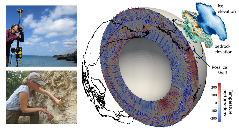
Figure: Reconstructing sea level in the field includes taking elevation measurements with high precision GPS (top left) and sampling corals for dating (bottom left). ASPECT was used to calculate mantle flow and associated topography changes at the surface to compare them to past sea level and couple it to Antarctic ice sheet reconstructions. The temperature perturbations is based on the S40RTS tomography model. Different slices of Antarctica denote the bedrock elevation (green – below sea level, brown – above sea level) and the elevation of the Antarctic ice sheet.